Variational autoencoder
Deep learning generative model to encode data representation


| Part of a series on |
| Machine learning and data mining |
|---|
| Paradigms
|
| Problems
|
| Learning with humans
|
| Model diagnostics
|
|
In machine learning, a variational autoencoder (VAE) is an artificial neural network architecture introduced by Diederik P. Kingma and Max Welling. It is part of the families of probabilistic graphical models and variational Bayesian methods.[1]
In addition to being seen as an autoencoder neural network architecture, variational autoencoders can also be studied within the mathematical formulation of variational Bayesian methods, connecting a neural encoder network to its decoder through a probabilistic latent space (for example, as a multivariate Gaussian distribution) that corresponds to the parameters of a variational distribution.
Thus, the encoder maps each point (such as an image) from a large complex dataset into a distribution within the latent space, rather than to a single point in that space. The decoder has the opposite function, which is to map from the latent space to the input space, again according to a distribution. By mapping a point to a distribution instead of a single point, the network can avoid overfitting the training data.[2] Both networks are typically trained together with the usage of the reparameterization trick, although the variance of the noise model can be learned separately.
Although this type of model was initially designed for unsupervised learning,[3][4] its effectiveness has been proven for semi-supervised learning[5][6] and supervised learning.[7]
Overview of architecture and operation
A variational autoencoder is a generative model with a prior and noise distribution respectively. Usually such models are trained using the expectation-maximization meta-algorithm (e.g. probabilistic PCA, (spike & slab) sparse coding). Such a scheme optimizes a lower bound of the data likelihood, which is usually intractable, and in doing so requires the discovery of q-distributions, or variational posteriors. These q-distributions are normally parameterized for each individual data point in a separate optimization process. However, variational autoencoders use a neural network as an amortized approach to jointly optimize across data points. This neural network takes as input the data points themselves, and outputs parameters for the variational distribution. As it maps from a known input space to the low-dimensional latent space, it is called the encoder.
The decoder is the second neural network of this model. It is a function that maps from the latent space to the input space, e.g. as the means of the noise distribution. It is possible to use another neural network that maps to the variance, however this can be omitted for simplicity. In such a case, the variance can be optimized with gradient descent.
To optimize this model, one needs to know two terms: the "reconstruction error", and the Kullback–Leibler divergence(KL-D). Both terms are derived from the free energy expression of the probabilistic model, and therefore differ depending on the noise distribution and the assumed prior of the data. For example, a standard VAE task such as IMAGENET is typically assumed to have a gaussianly distributed noise; however, tasks such as binarized MNIST require a Bernoulli noise. The KL-D from the free energy expression maximizes the probability mass of the q-distribution that overlaps with the p-distribution, which unfortunately can result in mode-seeking behaviour. The "reconstruction" term is the remainder of the free energy expression, and requires a sampling approximation to compute its expectation value.[8]
Formulation
From the point of view of probabilistic modeling, one wants to maximize the likelihood of the data by their chosen parameterized probability distribution . This distribution is usually chosen to be a Gaussian which is parameterized by and respectively, and as a member of the exponential family it is easy to work with as a noise distribution. Simple distributions are easy enough to maximize, however distributions where a prior is assumed over the latents results in intractable integrals. Let us find via marginalizing over .


where represents the joint distribution under of the observable data and its latent representation or encoding . According to the chain rule, the equation can be rewritten as


In the vanilla variational autoencoder, is usually taken to be a finite-dimensional vector of real numbers, and to be a Gaussian distribution. Then is a mixture of Gaussian distributions.

It is now possible to define the set of the relationships between the input data and its latent representation as
- Prior
- Likelihood
- Posterior


Unfortunately, the computation of is expensive and in most cases intractable. To speed up the calculus to make it feasible, it is necessary to introduce a further function to approximate the posterior distribution as

with defined as the set of real values that parametrize . This is sometimes called amortized inference, since by "investing" in finding a good , one can later infer from quickly without doing any integrals.


In this way, the problem is to find a good probabilistic autoencoder, in which the conditional likelihood distribution is computed by the probabilistic decoder, and the approximated posterior distribution is computed by the probabilistic encoder.

Parametrize the encoder as , and the decoder as .


Evidence lower bound (ELBO)
As in every deep learning problem, it is necessary to define a differentiable loss function in order to update the network weights through backpropagation.
For variational autoencoders, the idea is to jointly optimize the generative model parameters to reduce the reconstruction error between the input and the output, and to make as close as possible to . As reconstruction loss, mean squared error and cross entropy are often used.


As distance loss between the two distributions the Kullback–Leibler divergence is a good choice to squeeze under .[8][9]

The distance loss just defined is expanded as
![{\displaystyle {\begin{aligned}D_{KL}(q_{\phi }({z|x})\parallel p_{\theta }({z|x}))&=\mathbb {E} _{z\sim q_{\phi }(\cdot |x)}\left[\ln {\frac {q_{\phi }(z|x)}{p_{\theta }(z|x)}}\right]\\&=\mathbb {E} _{z\sim q_{\phi }(\cdot |x)}\left[\ln {\frac {q_{\phi }({z|x})p_{\theta }(x)}{p_{\theta }(x,z)}}\right]\\&=\ln p_{\theta }(x)+\mathbb {E} _{z\sim q_{\phi }(\cdot |x)}\left[\ln {\frac {q_{\phi }({z|x})}{p_{\theta }(x,z)}}\right]\end{aligned}}}](https://wikimedia.org/api/rest_v1/media/math/render/svg/12961b671abd2f6d9f8333b9fd2c69f5729452e6)
Now define the evidence lower bound (ELBO):
Maximizing the ELBO
![{\displaystyle L_{\theta ,\phi }(x):=\mathbb {E} _{z\sim q_{\phi }(\cdot |x)}\left[\ln {\frac {p_{\theta }(x,z)}{q_{\phi }({z|x})}}\right]=\ln p_{\theta }(x)-D_{KL}(q_{\phi }({\cdot |x})\parallel p_{\theta }({\cdot |x}))}](https://wikimedia.org/api/rest_v1/media/math/render/svg/f3930aaedee5df702f84e1571372c645eefa6572)
is equivalent to simultaneously maximizing and minimizing . That is, maximizing the log-likelihood of the observed data, and minimizing the divergence of the approximate posterior from the exact posterior .


The form given is not very convenient for maximization, but the following, equivalent form, is:
where is implemented as , since that is, up to an additive constant, what yields. That is, we model the distribution of conditional on to be a Gaussian distribution centered on . The distribution of and are often also chosen to be Gaussians as and , with which we obtain by the formula for KL divergence of Gaussians:
![{\displaystyle L_{\theta ,\phi }(x)=\mathbb {E} _{z\sim q_{\phi }(\cdot |x)}\left[\ln p_{\theta }(x|z)\right]-D_{KL}(q_{\phi }({\cdot |x})\parallel p_{\theta }(\cdot ))}](https://wikimedia.org/api/rest_v1/media/math/render/svg/e4ab2e155d237ffd569ef918817953a3ef82612c)


Here is the dimension of . For a more detailed derivation and more interpretations of ELBO and its maximization, see its main page.
![{\displaystyle L_{\theta ,\phi }(x)=-{\frac {1}{2}}\mathbb {E} _{z\sim q_{\phi }(\cdot |x)}\left[\|x-D_{\theta }(z)\|_{2}^{2}\right]-{\frac {1}{2}}\left(N\sigma _{\phi }(x)^{2}+\|E_{\phi }(x)\|_{2}^{2}-2N\ln \sigma _{\phi }(x)\right)+Const}](https://wikimedia.org/api/rest_v1/media/math/render/svg/166eb4fc2e504a10271e5bad8ba9fd0f69bc6de5)

Reparameterization


To efficiently search for
the typical method is gradient descent.
It is straightforward to find
However,
![{\displaystyle \nabla _{\theta }\mathbb {E} _{z\sim q_{\phi }(\cdot |x)}\left[\ln {\frac {p_{\theta }(x,z)}{q_{\phi }({z|x})}}\right]=\mathbb {E} _{z\sim q_{\phi }(\cdot |x)}\left[\nabla _{\theta }\ln {\frac {p_{\theta }(x,z)}{q_{\phi }({z|x})}}\right]}](https://wikimedia.org/api/rest_v1/media/math/render/svg/95305894e3cfbd10c985a9569091220891523aef)
does not allow one to put the inside the expectation, since appears in the probability distribution itself. The reparameterization trick (also known as stochastic backpropagation[10]) bypasses this difficulty.[8][11][12]
![{\displaystyle \nabla _{\phi }\mathbb {E} _{z\sim q_{\phi }(\cdot |x)}\left[\ln {\frac {p_{\theta }(x,z)}{q_{\phi }({z|x})}}\right]}](https://wikimedia.org/api/rest_v1/media/math/render/svg/bd826d47c8a9e4ac5fc59cef9026f401e9806df6)

The most important example is when is normally distributed, as .


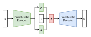
The scheme of a variational autoencoder after the reparameterization trick

This can be reparametrized by letting be a "standard random number generator", and construct as . Here, is obtained by the Cholesky decomposition:


Then we have

and so we obtained an unbiased estimator of the gradient, allowing stochastic gradient descent.
![{\displaystyle \nabla _{\phi }\mathbb {E} _{z\sim q_{\phi }(\cdot |x)}\left[\ln {\frac {p_{\theta }(x,z)}{q_{\phi }({z|x})}}\right]=\mathbb {E} _{\epsilon }\left[\nabla _{\phi }\ln {\frac {p_{\theta }(x,\mu _{\phi }(x)+L_{\phi }(x)\epsilon )}{q_{\phi }(\mu _{\phi }(x)+L_{\phi }(x)\epsilon |x)}}\right]}](https://wikimedia.org/api/rest_v1/media/math/render/svg/ab3c8e4238659d4273a37de83c8c40ce58c789fb)
Since we reparametrized , we need to find . Let be the probability density function for , then [clarification needed]


where is the Jacobian matrix of with respect to . Since , this is


Variations
Many variational autoencoders applications and extensions have been used to adapt the architecture to other domains and improve its performance.
-VAE is an implementation with a weighted Kullback–Leibler divergence term to automatically discover and interpret factorised latent representations. With this implementation, it is possible to force manifold disentanglement for values greater than one. This architecture can discover disentangled latent factors without supervision.[13][14]

The conditional VAE (CVAE), inserts label information in the latent space to force a deterministic constrained representation of the learned data.[15]
Some structures directly deal with the quality of the generated samples[16][17] or implement more than one latent space to further improve the representation learning.
Some architectures mix VAE and generative adversarial networks to obtain hybrid models.[18][19][20]
See also
References
- ^ Pinheiro Cinelli, Lucas; et al. (2021). "Variational Autoencoder". Variational Methods for Machine Learning with Applications to Deep Networks. Springer. pp. 111–149. doi:10.1007/978-3-030-70679-1_5. ISBN 978-3-030-70681-4. S2CID 240802776.
- ^ Rocca, Joseph (2021-03-21). "Understanding Variational Autoencoders (VAEs)". Medium.
- ^ Dilokthanakul, Nat; Mediano, Pedro A. M.; Garnelo, Marta; Lee, Matthew C. H.; Salimbeni, Hugh; Arulkumaran, Kai; Shanahan, Murray (2017-01-13). "Deep Unsupervised Clustering with Gaussian Mixture Variational Autoencoders". arXiv:1611.02648 [cs.LG].
- ^ Hsu, Wei-Ning; Zhang, Yu; Glass, James (December 2017). "Unsupervised domain adaptation for robust speech recognition via variational autoencoder-based data augmentation". 2017 IEEE Automatic Speech Recognition and Understanding Workshop (ASRU). pp. 16–23. arXiv:1707.06265. doi:10.1109/ASRU.2017.8268911. ISBN 978-1-5090-4788-8. S2CID 22681625.
- ^ Ehsan Abbasnejad, M.; Dick, Anthony; van den Hengel, Anton (2017). Infinite Variational Autoencoder for Semi-Supervised Learning. pp. 5888–5897.
- ^ Xu, Weidi; Sun, Haoze; Deng, Chao; Tan, Ying (2017-02-12). "Variational Autoencoder for Semi-Supervised Text Classification". Proceedings of the AAAI Conference on Artificial Intelligence. 31 (1). doi:10.1609/aaai.v31i1.10966. S2CID 2060721.
- ^ Kameoka, Hirokazu; Li, Li; Inoue, Shota; Makino, Shoji (2019-09-01). "Supervised Determined Source Separation with Multichannel Variational Autoencoder". Neural Computation. 31 (9): 1891–1914. doi:10.1162/neco_a_01217. PMID 31335290. S2CID 198168155.
- ^ a b c Kingma, Diederik P.; Welling, Max (2013-12-20). "Auto-Encoding Variational Bayes". arXiv:1312.6114 [stat.ML].
- ^ "From Autoencoder to Beta-VAE". Lil'Log. 2018-08-12.
- ^ Rezende, Danilo Jimenez; Mohamed, Shakir; Wierstra, Daan (2014-06-18). "Stochastic Backpropagation and Approximate Inference in Deep Generative Models". International Conference on Machine Learning. PMLR: 1278–1286. arXiv:1401.4082.
- ^ Bengio, Yoshua; Courville, Aaron; Vincent, Pascal (2013). "Representation Learning: A Review and New Perspectives". IEEE Transactions on Pattern Analysis and Machine Intelligence. 35 (8): 1798–1828. arXiv:1206.5538. doi:10.1109/TPAMI.2013.50. ISSN 1939-3539. PMID 23787338. S2CID 393948.
- ^ Kingma, Diederik P.; Rezende, Danilo J.; Mohamed, Shakir; Welling, Max (2014-10-31). "Semi-Supervised Learning with Deep Generative Models". arXiv:1406.5298 [cs.LG].
- ^ Higgins, Irina; Matthey, Loic; Pal, Arka; Burgess, Christopher; Glorot, Xavier; Botvinick, Matthew; Mohamed, Shakir; Lerchner, Alexander (2016-11-04). "beta-VAE: Learning Basic Visual Concepts with a Constrained Variational Framework".
{{cite journal}}: Cite journal requires|journal=(help) - ^ Burgess, Christopher P.; Higgins, Irina; Pal, Arka; Matthey, Loic; Watters, Nick; Desjardins, Guillaume; Lerchner, Alexander (2018-04-10). "Understanding disentangling in β-VAE". arXiv:1804.03599 [stat.ML].
- ^ Sohn, Kihyuk; Lee, Honglak; Yan, Xinchen (2015-01-01). "Learning Structured Output Representation using Deep Conditional Generative Models" (PDF).
{{cite journal}}: Cite journal requires|journal=(help) - ^ Dai, Bin; Wipf, David (2019-10-30). "Diagnosing and Enhancing VAE Models". arXiv:1903.05789 [cs.LG].
- ^ Dorta, Garoe; Vicente, Sara; Agapito, Lourdes; Campbell, Neill D. F.; Simpson, Ivor (2018-07-31). "Training VAEs Under Structured Residuals". arXiv:1804.01050 [stat.ML].
- ^ Larsen, Anders Boesen Lindbo; Sønderby, Søren Kaae; Larochelle, Hugo; Winther, Ole (2016-06-11). "Autoencoding beyond pixels using a learned similarity metric". International Conference on Machine Learning. PMLR: 1558–1566. arXiv:1512.09300.
- ^ Bao, Jianmin; Chen, Dong; Wen, Fang; Li, Houqiang; Hua, Gang (2017). "CVAE-GAN: Fine-Grained Image Generation Through Asymmetric Training". pp. 2745–2754. arXiv:1703.10155 [cs.CV].
- ^ Gao, Rui; Hou, Xingsong; Qin, Jie; Chen, Jiaxin; Liu, Li; Zhu, Fan; Zhang, Zhao; Shao, Ling (2020). "Zero-VAE-GAN: Generating Unseen Features for Generalized and Transductive Zero-Shot Learning". IEEE Transactions on Image Processing. 29: 3665–3680. Bibcode:2020ITIP...29.3665G. doi:10.1109/TIP.2020.2964429. ISSN 1941-0042. PMID 31940538. S2CID 210334032.


