Spiral optimization algorithm
Optimization algorithm
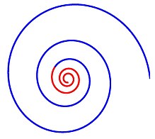
The spiral shares the global (blue) and intensive (red) behavior

In mathematics, the spiral optimization (SPO) algorithm is a metaheuristic inspired by spiral phenomena in nature.

The first SPO algorithm was proposed for two-dimensional unconstrained optimization[1] based on two-dimensional spiral models. This was extended to n-dimensional problems by generalizing the two-dimensional spiral model to an n-dimensional spiral model.[2] There are effective settings for the SPO algorithm: the periodic descent direction setting[3] and the convergence setting.[4]

Metaphor

The motivation for focusing on spiral phenomena was due to the insight that the dynamics that generate logarithmic spirals share the diversification and intensification behavior. The diversification behavior can work for a global search (exploration) and the intensification behavior enables an intensive search around a current found good solution (exploitation).

Algorithm
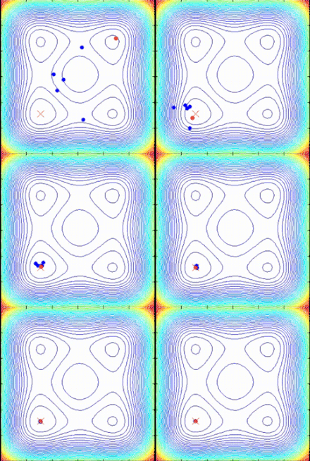
Spiral Optimization (SPO) algorithm

The SPO algorithm is a multipoint search algorithm that has no objective function gradient, which uses multiple spiral models that can be described as deterministic dynamical systems. As search points follow logarithmic spiral trajectories towards the common center, defined as the current best point, better solutions can be found and the common center can be updated.

The general SPO algorithm for a minimization problem under the maximum iteration k max {\displaystyle k_{\max }} (termination criterion) is as follows:

0) Set the number of search points 


        m
        
        2
      
    
    {\displaystyle m\geq 2}
  
 and the maximum iteration number 


          k
          
            max


    {\displaystyle k_{\max }}
  
.
1) Place the initial search points 


          x
          
            i
          
        
        (
        0
        )


            R
          
          
            n


        (
        i
        =
        1
        ,
        
        ,
        m
        )
      
    
    {\displaystyle x_{i}(0)\in \mathbb {R} ^{n}~(i=1,\ldots ,m)}
  
 and determine the center 


          x


        (
        0
        )
        =
        
          x
          
            
              i
              
                b


        (
        0
        )
      
    
    {\displaystyle x^{\star }(0)=x_{i_{\text{b}}}(0)}
  
, 


            i
            
              b
            
          
          =
          
            
              argmin
            
            
              i
              =
              1
              ,
              
              ,
              m


          {
          f
          (
          
            x
            
              i
            
          
          (
          0
          )
          )
          }


    {\displaystyle \displaystyle i_{\text{b}}=\mathop {\text{argmin}} _{i=1,\ldots ,m}\{f(x_{i}(0))\}}
  
,and then set 


        k
        =
        0
      
    
    {\displaystyle k=0}
  
.
2) Decide the step rate 


        r
        (
        k
        )
      
    
    {\displaystyle r(k)}
  
 by a rule.
3) Update the search points: 


          x
          
            i
          
        
        (
        k
        +
        1
        )
        =
        
          x


        (
        k
        )
        +
        r
        (
        k
        )
        R
        (
        θ
        )
        (
        
          x
          
            i
          
        
        (
        k
        )
        
        
          x


        (
        k
        )
        )
        
        (
        i
        =
        1
        ,
        
        ,
        m
        )
        .
      
    
    {\displaystyle x_{i}(k+1)=x^{\star }(k)+r(k)R(\theta )(x_{i}(k)-x^{\star }(k))\quad (i=1,\ldots ,m).}
  

4) Update the center: 


          x


        (
        k
        +
        1
        )
        =
        
          
            {


                    x
                    
                      
                        i
                        
                          b


                  (
                  k
                  +
                  1
                  )


                      (


                    if 
                  
                  f
                  (
                  
                    x
                    
                      
                        i
                        
                          b


                  (
                  k
                  +
                  1
                  )
                  )
                  <
                  f
                  (
                  
                    x


                  (
                  k
                  )
                  )
                  
                    
                      )
                    
                  
                  ,


                    x


                  (
                  k
                  )


                      (


                    otherwise


                      )
                    
                  
                  ,


    {\displaystyle x^{\star }(k+1)={\begin{cases}x_{i_{\text{b}}}(k+1)&{\big (}{\text{if }}f(x_{i_{\text{b}}}(k+1))<f(x^{\star }(k)){\big )},\\x^{\star }(k)&{\big (}{\text{otherwise}}{\big )},\end{cases}}}
  
 where 


            i
            
              b
            
          
          =
          
            
              argmin
            
            
              i
              =
              1
              ,
              
              ,
              m


          {
          f
          (
          
            x
            
              i
            
          
          (
          k
          +
          1
          )
          )
          }


    {\displaystyle \displaystyle i_{\text{b}}=\mathop {\text{argmin}} _{i=1,\ldots ,m}\{f(x_{i}(k+1))\}}
  
.
5) Set 


        k
        :=
        k
        +
        1
      
    
    {\displaystyle k:=k+1}
  
. If 


        k
        =
        
          k
          
            max


    {\displaystyle k=k_{\max }}
  
 is satisfied then terminate and output 


          x


        (
        k
        )
      
    
    {\displaystyle x^{\star }(k)}
  
. Otherwise, return to Step 2).

Setting

The search performance depends on setting the composite rotation matrix R ( θ ) {\displaystyle R(\theta )} , the step rate r ( k ) {\displaystyle r(k)} , and the initial points x i ( 0 )   ( i = 1 , , m ) {\displaystyle x_{i}(0)~(i=1,\ldots ,m)} . The following settings are new and effective.

Setting 1 (Periodic Descent Direction Setting)

This setting is an effective setting for high dimensional problems under the maximum iteration k max {\displaystyle k_{\max }} . The conditions on R ( θ ) {\displaystyle R(\theta )} and x i ( 0 )   ( i = 1 , , m ) {\displaystyle x_{i}(0)~(i=1,\ldots ,m)} together ensure that the spiral models generate descent directions periodically. The condition of r ( k ) {\displaystyle r(k)} works to utilize the periodic descent directions under the search termination k max {\displaystyle k_{\max }} .

  • Set R ( θ ) {\displaystyle R(\theta )} as follows: R ( θ ) = [ 0 n 1 1 I n 1 0 n 1 ] {\displaystyle R(\theta )={\begin{bmatrix}0_{n-1}^{\top }&-1\\I_{n-1}&0_{n-1}\\\end{bmatrix}}} where I n 1 {\displaystyle I_{n-1}} is the ( n 1 ) × ( n 1 ) {\displaystyle (n-1)\times (n-1)} identity matrix and 0 n 1 {\displaystyle 0_{n-1}} is the ( n 1 ) × 1 {\displaystyle (n-1)\times 1} zero vector.
  • Place the initial points x i ( 0 ) R n {\displaystyle x_{i}(0)\in \mathbb {R} ^{n}} ( i = 1 , , m ) {\displaystyle (i=1,\ldots ,m)} at random to satisfy the following condition:

min i = 1 , , m { max j = 1 , , m { rank [ d j , i ( 0 )   R ( θ ) d j , i ( 0 )         R ( θ ) 2 n 1 d j , i ( 0 ) ] } } = n {\displaystyle \min _{i=1,\ldots ,m}\{\max _{j=1,\ldots ,m}{\bigl \{}{\text{rank}}{\bigl [}d_{j,i}(0)~R(\theta )d_{j,i}(0)~~\cdots ~~R(\theta )^{2n-1}d_{j,i}(0){\bigr ]}{\bigr \}}{\bigr \}}=n} where d j , i ( 0 ) = x j ( 0 ) x i ( 0 ) {\displaystyle d_{j,i}(0)=x_{j}(0)-x_{i}(0)} . Note that this condition is almost all satisfied by a random placing and thus no check is actually fine.

  • Set r ( k ) {\displaystyle r(k)} at Step 2) as follows: r ( k ) = r = δ k max         (constant value) {\displaystyle r(k)=r={\sqrt[{k_{\max }}]{\delta }}~~~~{\text{(constant value)}}} where a sufficiently small δ > 0 {\displaystyle \delta >0} such as δ = 1 / k max {\displaystyle \delta =1/k_{\max }} or δ = 10 3 {\displaystyle \delta =10^{-3}} .[3]

Setting 2 (Convergence Setting)

This setting ensures that the SPO algorithm converges to a stationary point under the maximum iteration k max = {\displaystyle k_{\max }=\infty } . The settings of R ( θ ) {\displaystyle R(\theta )} and the initial points x i ( 0 )   ( i = 1 , , m ) {\displaystyle x_{i}(0)~(i=1,\ldots ,m)} are the same with the above Setting 1. The setting of r ( k ) {\displaystyle r(k)} is as follows.

  • Set r ( k ) {\displaystyle r(k)} at Step 2) as follows: r ( k ) = { 1 ( k k k + 2 n 1 ) , h ( k k + 2 n ) , {\displaystyle r(k)={\begin{cases}1&(k^{\star }\leqq k\leqq k^{\star }+2n-1),\\h&(k\geqq k^{\star }+2n),\end{cases}}} where k {\displaystyle k^{\star }} is an iteration when the center is newly updated at Step 4) and h = δ 2 n , δ ( 0 , 1 ) {\displaystyle h={\sqrt[{2n}]{\delta }},\delta \in (0,1)} such as δ = 0.5 {\displaystyle \delta =0.5} . Thus we have to add the following rules about k {\displaystyle k^{\star }} to the Algorithm:
•(Step 1) k = 0 {\displaystyle k^{\star }=0} .
•(Step 4) If x ( k + 1 ) x ( k ) {\displaystyle x^{\star }(k+1)\neq x^{\star }(k)} then k = k + 1 {\displaystyle k^{\star }=k+1} .[4]

Future works

  • The algorithms with the above settings are deterministic. Thus, incorporating some random operations make this algorithm powerful for global optimization. Cruz-Duarte et al.[5] demonstrated it by including stochastic disturbances in spiral searching trajectories. However, this door remains open to further studies.
  • To find an appropriate balance between diversification and intensification spirals depending on the target problem class (including k max {\displaystyle k_{\max }} ) is important to enhance the performance.

Extended works

Many extended studies have been conducted on the SPO due to its simple structure and concept; these studies have helped improve its global search performance and proposed novel applications.[6][7][8][9][10][11]

References

  1. ^ Tamura, K.; Yasuda, K. (2011). "Primary Study of Spiral Dynamics Inspired Optimization". IEEJ Transactions on Electrical and Electronic Engineering. 6 (S1): 98–100. doi:10.1002/tee.20628. S2CID 109093423.
  2. ^ Tamura, K.; Yasuda, K. (2011). "Spiral Dynamics Inspired Optimization". Journal of Advanced Computational Intelligence and Intelligent Informatics. 132 (5): 1116–1121. doi:10.20965/jaciii.2011.p1116.
  3. ^ a b Tamura, K.; Yasuda, K. (2016). "Spiral Optimization Algorithm Using Periodic Descent Directions". SICE Journal of Control, Measurement, and System Integration. 6 (3): 133–143. Bibcode:2016JCMSI...9..134T. doi:10.9746/jcmsi.9.134.
  4. ^ a b Tamura, K.; Yasuda, K. (2020). "The Spiral Optimization Algorithm: Convergence Conditions and Settings". IEEE Transactions on Systems, Man, and Cybernetics: Systems. 50 (1): 360–375. doi:10.1109/TSMC.2017.2695577. S2CID 126109444.
  5. ^ Cruz-Duarte, Jorge M.; Martin-Diaz, Ignacio; Munoz-Minjares, J. U.; Sanchez-Galindo, Luis A.; Avina-Cervantes, Juan G.; Garcia-Perez, Arturo; Correa-Cely, C. Rodrigo (2017). "Primary study on the stochastic spiral optimization algorithm". 2017 IEEE International Autumn Meeting on Power, Electronics and Computing (ROPEC). pp. 1–6. doi:10.1109/ROPEC.2017.8261609. ISBN 978-1-5386-0819-7. S2CID 37580653.
  6. ^ Nasir, A. N. K.; Tokhi, M. O. (2015). "An improved spiral dynamic optimization algorithm with engineering application". IEEE Transactions on Systems, Man, and Cybernetics: Systems. 45 (6): 943–954. doi:10.1109/tsmc.2014.2383995. S2CID 24253496.
  7. ^ Nasir, A. N. K.; Ismail, R.M.T.R.; Tokhi, M. O. (2016). "Adaptive spiral dynamics metaheuristic algorithm for global optimisation with application to modelling of a flexible system" (PDF). Applied Mathematical Modelling. 40 (9–10): 5442–5461. doi:10.1016/j.apm.2016.01.002.
  8. ^ Ouadi, A.; Bentarzi, H.; Recioui, A. (2013). "multiobjective design of digital filters using spiral optimization technique". SpringerPlus. 2 (461): 697–707. doi:10.1186/2193-1801-2-461. PMC 3786071. PMID 24083108.
  9. ^ Benasla, L.; Belmadani, A.; Rahli, M. (2014). "Spiral optimization algorithm for solving combined economic and Emission Dispatch". International Journal of Electrical Power & Energy Systems. 62: 163–174. doi:10.1016/j.ijepes.2014.04.037.
  10. ^ Sidarto, K. A.; Kania, A. (2015). "Finding all solutions of systems of nonlinear equations using spiral dynamics inspired optimization with clustering". Journal of Advanced Computational Intelligence and Intelligent Informatics. 19 (5): 697–707. doi:10.20965/jaciii.2015.p0697.
  11. ^ Kaveh, A.; Mahjoubi, S. (October 2019). "Hypotrochoid spiral optimization approach for sizing and layout optimization of truss structures with multiple frequency constraints". Engineering with Computers. 35 (4): 1443–1462. doi:10.1007/s00366-018-0675-6. S2CID 54457145.
  • v
  • t
  • e
Optimization: Algorithms, methods, and heuristics
Unconstrained nonlinear
Functions
Gradients
Convergence
Quasi–Newton
Other methods
Hessians
Graph of a strictly concave quadratic function with unique maximum.
Optimization computes maxima and minima.
General
Differentiable
Convex
minimization
Linear and
quadratic
Interior point
Basis-exchange
Paradigms
Graph
algorithms
Minimum
spanning tree
Shortest path
Network flows